파이썬 랜덤(Random) 뽑기 - 로그노멀분포, 파레토분포, 웨이블분포

 

 

 

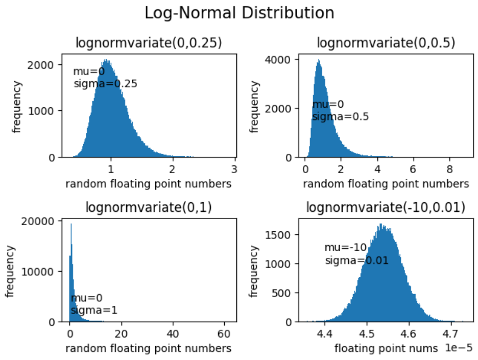
로그노멀(Log-Normal)분포 난수 생성 방법

random.lognormvariate(mu, sigma) 함수 사용

로그노멀 분포에 자연로그를 취하면 평균 mu에 표준편차 sigma를 갖는 정규분포가 됨

로그노멀분포 난수 생성

 

위키피디아 로그노멀분포: 
https://en.wikipedia.org/wiki/Log-normal_distribution

Log-normal distribution - Wikipedia

 

로그노멀분포 생성 및 시각화:

import random as r
import matplotlib.pyplot as plt

# 로그-노멀분포(Log-Normal Distribution) 난수 생성 

fig, axs = plt.subplots(nrows=2, ncols=2)

# 1. mu = 0, sigma = 0.25 인 경우 
m = 0
s = 0.25
rand = [r.lognormvariate(mu=m, sigma=s) for i in range(100000)] 
plt.subplot(221)
plt.hist(rand, bins=200)
ax = plt.gca()
ax.set_xlabel("random floating point numbers")
ax.set_ylabel("frequency")
plt.title("lognormvariate("+str(m)+","+str(s)+")")
ax.text(x=0.4, y=1500, s="mu="+str(m)+"\n"+"sigma="+str(s))

# 1. mu = 0, sigma = 0.25 인 경우 
m = 0
s = 0.5
rand = [r.lognormvariate(mu=m, sigma=s) for i in range(100000)] 
plt.subplot(222)
plt.hist(rand, bins=200)
ax = plt.gca()
ax.set_xlabel("random floating point numbers")
ax.set_ylabel("frequency")
plt.title("lognormvariate("+str(m)+","+str(s)+")")
ax.text(x=0.4, y=1500, s="mu="+str(m)+"\n"+"sigma="+str(s))

# 1. mu = 0, sigma = 0.25 인 경우 
m = 0
s = 1
rand = [r.lognormvariate(mu=m, sigma=s) for i in range(100000)] 
plt.subplot(223)
plt.hist(rand, bins=200)
ax = plt.gca()
ax.set_xlabel("random floating point numbers")
ax.set_ylabel("frequency")
plt.title("lognormvariate("+str(m)+","+str(s)+")")
ax.text(x=0.4, y=1500, s="mu="+str(m)+"\n"+"sigma="+str(s))

# 1. mu = 0, sigma = 0.25 인 경우 
m = -10
s = 0.01
rand = [r.lognormvariate(mu=m, sigma=s) for i in range(100000)] 
plt.subplot(224)
plt.hist(rand, bins=200)
ax = plt.gca()
ax.set_xlabel("floating point nums")
ax.set_ylabel("frequency")
plt.title("lognormvariate("+str(m)+","+str(s)+")")
ax.text(x=0.000044, y=1000, s="mu="+str(m)+"\n"+"sigma="+str(s))

fig.suptitle("Log-Normal Distribution", fontsize=15)
plt.tight_layout()

 

 

 

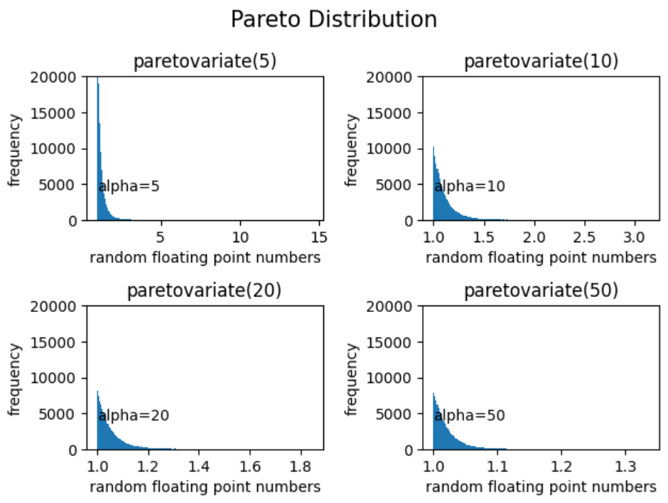
파레토(Pareto)분포 난수 생성 방법

random. paretovariate (alpha) 함수 사용

파레토 분포 난수 생성

 

위키피디아 파레토분포: 

https://en.wikipedia.org/wiki/Pareto_distribution

Pareto distribution - Wikipedia

 

파레토 분포 난수 생성 및 시각화: 

import random as r
import matplotlib.pyplot as plt
import numpy as np

# 파레토 분포(Pareto Distribution) 난수 생성 

fig, axs = plt.subplots(nrows=2, ncols=2)
ylim = 20000

# 1. alpha = 5 인 경우 
a = 5
rand = [r.paretovariate(alpha=a) for i in range(100000)] 
plt.subplot(221)
plt.hist(rand, bins=200)
ax = plt.gca()
ax.set_xlabel("random floating point numbers")
ax.set_ylabel("frequency")
ax.set_ylim(0,ylim)
plt.title("paretovariate("+str(a)+")")
ax.text(x=1, y=4000, s="alpha="+str(a))

# 2. alpha = 10 인 경우 
a = 10
rand = [r.paretovariate(alpha=a) for i in range(100000)] 
plt.subplot(222)
plt.hist(rand, bins=200)
ax = plt.gca()
ax.set_xlabel("random floating point numbers")
ax.set_ylabel("frequency")
ax.set_ylim(0,ylim)
plt.title("paretovariate("+str(a)+")")
ax.text(x=1, y=4000, s="alpha="+str(a))

# 3. alpha = 20 인 경우 
a = 20
rand = [r.paretovariate(alpha=a) for i in range(100000)] 
plt.subplot(223)
plt.hist(rand, bins=200)
ax = plt.gca()
ax.set_xlabel("random floating point numbers")
ax.set_ylabel("frequency")
ax.set_ylim(0,ylim)
plt.title("paretovariate("+str(a)+")")
ax.text(x=1, y=4000, s="alpha="+str(a))

# 4. alpha = 50 인 경우 
a = 50
rand = [r.paretovariate(alpha=a) for i in range(100000)] 
plt.subplot(224)
plt.hist(rand, bins=200)
ax = plt.gca()
ax.set_xlabel("random floating point numbers")
ax.set_ylabel("frequency")
ax.set_ylim(0,ylim)
plt.title("paretovariate("+str(a)+")")
ax.text(x=1, y=4000, s="alpha="+str(a))

fig.suptitle("Pareto Distribution", fontsize=15)
plt.tight_layout()

 

 

 

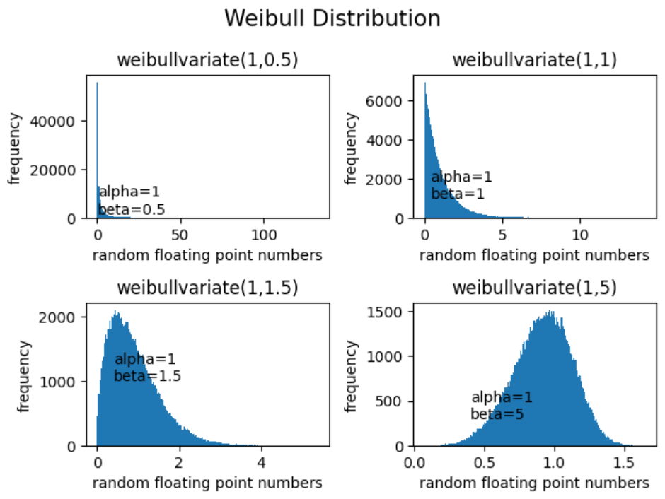
웨이블(Weibull)분포 난수 생성 방법

random. weibullvariate(alpha, beta) 함수 사용

고장모드, 신뢰성 분석에 많이 사용함

웨이블 분포 난수 생성

 

위키피디아 웨이블분포: 

https://en.wikipedia.org/wiki/Weibull_distribution

Weibull distribution - Wikipedia

 

웨이블 분포 난수 생성 및 시각화:

import random as r
import matplotlib.pyplot as plt

# 웨이블 분포 (Weibull Distribution) 난수 생성

fig, axs = plt.subplots(nrows=2, ncols=2)

# 1. alpha = beta = 0.5 인 경우 
a = 1
b = 0.5
rand = [r.weibullvariate(alpha=a,beta=b) for i in range(100000)] 
plt.subplot(221)
plt.hist(rand, bins=200)
ax = plt.gca()
ax.set_xlabel("random floating point numbers")
ax.set_ylabel("frequency")
plt.title("weibullvariate("+str(a)+","+str(b)+")")
ax.text(x=0.4, y=1500, s="alpha="+str(a)+"\n"+"beta="+str(b))

# 2. alpha =5, beta =1 
a = 1
b = 1
rand = [r.weibullvariate(alpha=a,beta=b) for i in range(100000)] 
plt.subplot(222)
plt.hist(rand, bins=200)
ax = plt.gca()
ax.set_xlabel("random floating point numbers")
ax.set_ylabel("frequency")
plt.title("weibullvariate("+str(a)+","+str(b)+")")
ax.text(x=0.4, y=1000, s="alpha="+str(a)+"\n"+"beta="+str(b))

# 3. alpha =1, beta =3 
a = 1
b = 1.5
rand = [r.weibullvariate(alpha=a,beta=b) for i in range(100000)] 
plt.subplot(223)
plt.hist(rand, bins=200)
ax = plt.gca()
ax.set_xlabel("random floating point numbers")
ax.set_ylabel("frequency")
plt.title("weibullvariate("+str(a)+","+str(b)+")")
ax.text(x=0.4, y=1000, s="alpha="+str(a)+"\n"+"beta="+str(b))

# 4. alpha =2, beta =2 
a = 1
b = 5
rand = [r.weibullvariate(alpha=a,beta=b) for i in range(100000)] 
plt.subplot(224)
plt.hist(rand, bins=200)
ax = plt.gca()
ax.set_xlabel("random floating point numbers")
ax.set_ylabel("frequency")
plt.title("weibullvariate("+str(a)+","+str(b)+")")
ax.text(x=0.4, y=300, s="alpha="+str(a)+"\n"+"beta="+str(b))

fig.suptitle("Weibull Distribution", fontsize=15)
plt.tight_layout()